Most of the off-the-shelf tools of data analysis of time series rely on homogeneity of the time line (i.e. the fact that time considered as homogeneous space of $\Real$ as a group).
This implicit assumption underlies all versions of Fourier analysis, and a lot of other tools in statistics and beyond.

It mostly is satisfied in physical systems, but fails spectacularly in biological, economic, social ones.

This research thread grew out of question what principled tools of data analysis are there, that are reparameterization invariant.
In other words, we are looking for functionals $I$ on the space of (continuous) trajectories \[ \paths=\{\path:I\to V, I=[0,T], V\cong \Real^d\} \] that survive reparametrization of the timeline: \[ I(\path)=I(\path\circ \tau), \tau:I\to I. \]

Remarkably, all such functionals have been shown by K.-T. Chen to be iterated integrals.

Iterated integrals are functions of a path $I(\path)$ forming a vector space filtered by their order, and are defined as follows:

• The iterated integrals of order $0$ of a path $\path_t:[0,t]\to V$ are just constants.
• If $I$ is an iterated integral of order $k$, then the functional \[ I(\path_t):=\int_0^t I(\path_s)d\path_k(s) \] is an iterated integral of order $(k+1)$. (Here $\path_k$ is the $k$-th component of $\path=(\path_1,\ldots,\path_d)$.)

For example, the iterated integrals of order $1$ are increments along the path.

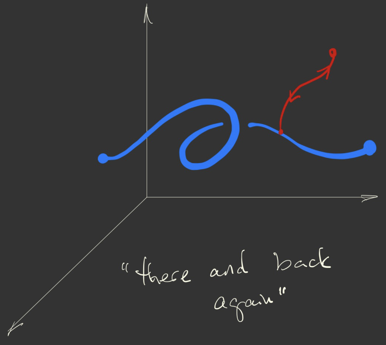
One complication is that the iterated integrals don't change if one inserts a detour, a path immediately followed by its inverse. If a path does not contain a detour, we will call it irreducible.

Then one has the following

Theorem(K.-T. Chen, '58) Two irreducible paths with the same starting point and iterated integrals of all orders are related by a reparameterization.

Often one writes iterated integrals of order $k$ as \[ \int_{0\lt t_1\lt t_2\lt \cdots\lt t_k\lt t}df_{l_1}(t_1) \ldots df_{l_k}(t). \]

Iterated integrals have many nice properties: they also appear as Picard approximations in elementary theory of ODEs, as Wiener chaos expansions, as Kontsevich integrals for finite type knot invariants... The dimensions of the elements of the filtration are same as those of free nilpotent Lie algebras,...

We won't be talking here about any of those.

We adopt a dogmatic view: if a phenomenon is not intrinsically clocked, one needs to use reparametrization invariant descriptors.

Terry Lyons pursued the idea to use iterated integrals for data analysis. His approach is to take the totality of them (signatures) and use them as a full descriptor. Our approach goes in a completely different direction.

In this story we focus on iterated integrals of order two.

Iterated integrals of order two (aside from squares of the increments) are spanned by the oriented areas of projections of the trajectories to 2-planes in $\Real^d$.
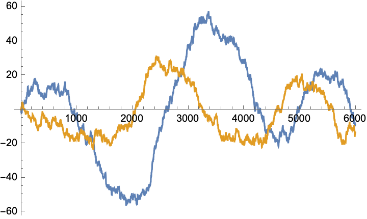
We use these oriented area as a heuristic measure of the Lead-Lag relationship between components of a time series.

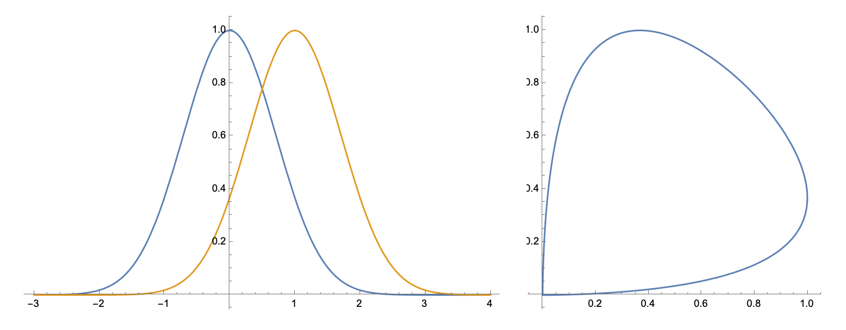
The pair of time series below form a lead/follow pair. This manifests in the positive oriented area circumscribed by the parametric curve. (There is some ambiguity in calibration of this area if the path is not closed; we always close it by a straight segment.)

In $d$-dimensional paths, we assemble these oriented areas into the $d\times d$ real skew-symmetric matrix $A$ we dub the lead matrix: \[ A_{kl}=\frac12\int_0^T x_k(t)dx_l(t)-x_l(t)d x_k(t). \]

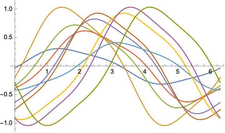
Consider a class of models that plausibly describe many cyclic yet not periodic phenomena.

Assume that internal clock is $S^1\cong \Real/P\Int$, and that time series functions of the internal clock related by shift and rescaling: \[ x_k(\tau)=c_k\phi(\tau-\alpha_k), c_k>0. \] The offsets $\alpha_k, k=1,\ldots,d$ define the cyclic order of the observables $x_k$.

In physical time, the observations are \( x_k(t)=x_k(\mathbf{\tau}(t))x \) where $\mathbf{\tau}:\Real\to S^1$ is some covering.

We will refer to this model as COOM, the Chain of Offsets Model.

If one forms lead matrix for such a process (over one cycle), its components are given by \[ A_{kl}=\psi(\alpha_k-\alpha_l), \] where \[ \psi=(\phi*\phi^\circ)', \] the derivative of the convolution of $\phi$ with its time-reversed version.

If $\phi\equiv \sin$, one can derive that the lead matrix has rank $2$, and the components of the nontrivial eigenvector are obtained from \[ v_k=c_k\exp(i\alpha_k) \] by an $\Real$-linear transformation of the complex plane.

Therefore, the cyclic order defined by the arguments of these components is the same as the cyclic order of \(\exp(i\alpha_k)\).

This suggests a heuristic computational pipe for recovery of the cyclic order of the observables under COOM.

We will discuss examples of the recovery of cyclic order later.

A version of the COOM emerges when one considers not cycles, but waves: say, linear array of sensors excited consecutively.

Similarly to the cyclic case, one arrives to the skew symmetric Toeplitz matrices, and the leading eigenvector still reflects the adjacencies of the sensors, but in more convoluted fashion.

(This can be derived from some results of Böttcher, Grudsky, Unterberger,...).

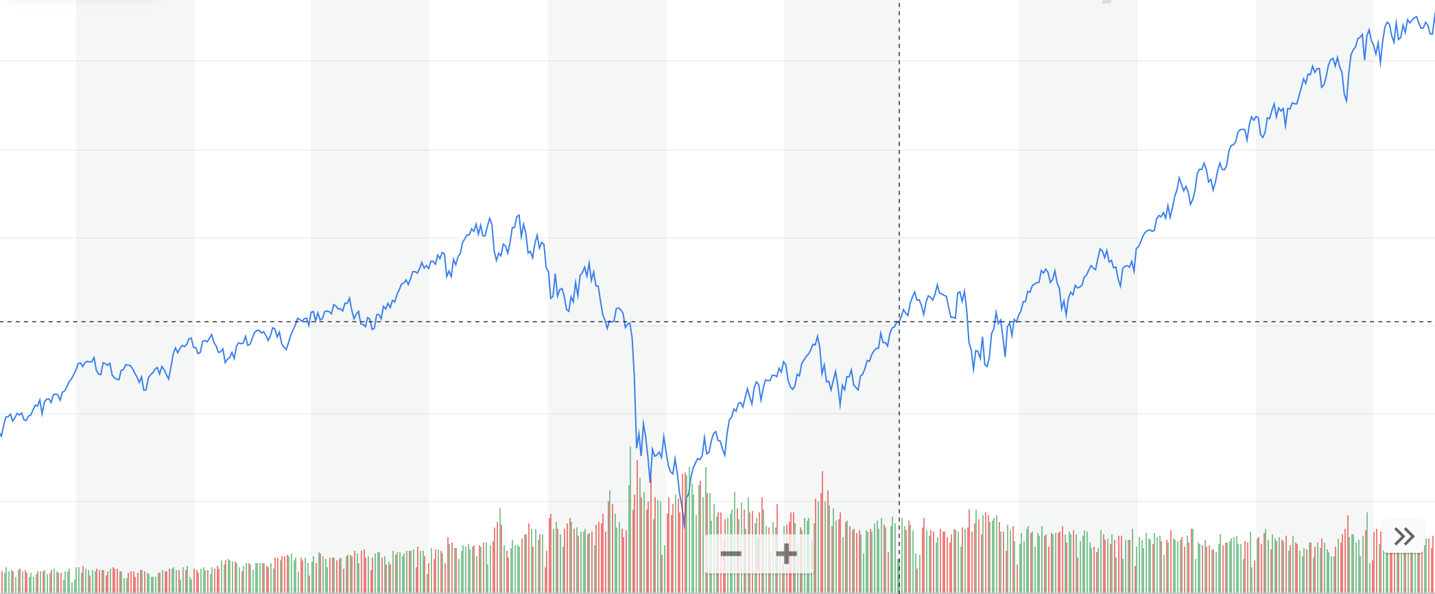
The US economy goes through highly aperiodic cycles of business activity. At the aggregate level, the key indicator is the GDP growth, but many correlates of the business activity exist, most notably, the unemployment data, bonds returns etc.

The data are notoriously noisy.

Investors long sought to exploit the dependences of the stock returns on the stages of the business cycle.

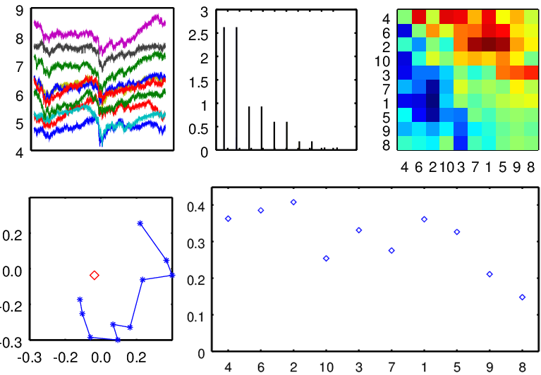
We considered the sectorial indices (as reported by Standard and Poor) for the daily closings, over a period of 2003-2016.

These are the aggregates corresponding to the subsets of stock values tracked by S&P as a part of their industrial portfolio.

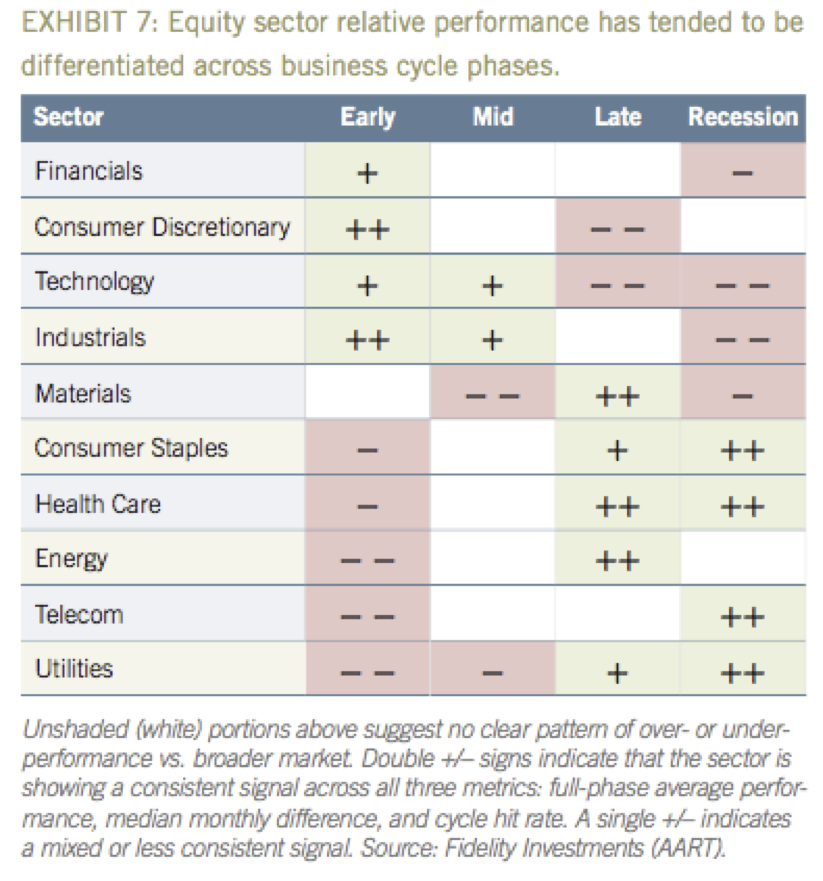
It is "well known" that these industrial sectors exhibit some kind of cyclic behavior (some showing better returns at the start of a business cycle; others - towards its end).

Here are the ten industrial sectors, each an aggregate of several publically traded companies, and an excerpt from a Fidelity investment guide:

BM Materials CY Consumer Cyclical EN Energy FN Financial HC Health Care IN Industrials NC Consumer Staples (Non-Cyclical) TC Technology TL Telecommunications UT Utilities

Assuming the chain of offset model, we analyzed these time series of the industrial sectors. The data were downloaded from finance.google.com, $\log$-ed, detrended and normalized. The results are shown below.

The resulting (cyclic) order, shown below, is in a close agreement with the financial "folklore knowledge":

Let's investigate how our computational pipe would perform on a model or a noisy cyclic system \[ d\bx=R\bx dt+Bd\bw; \] here $\bx\in V\cong \Real^d$, $R\in\mat(d\times d,\Real), B\in \mat(d\times l,\Real)$ and $\bw=(w_1,\ldots,w_l)$ is a collection of standard uncorrelated Brownian motions.

In "controllable case" (when no $R$-invariant subspace contains the range of $B$), and $R$ is Hurwitz (all eigenvalues in the left halfplane), the stationary distribution has Gaussian density \[ p(\bx)=Z^{-1}e^{-(S^{-1}\bx,\bx)/2}, \] where covariance $S$ solved the Sylvester-Lyapunov equation $RS+SR^\dagger=BB^\dagger=:\Sigma$.

The distribution might be stationary, but in general the stochastic dynamics results in a nontrivial flux:

Simulated evolution for the system with \[ R=\begin{pmatrix} -1&.4\\-.1&-1\\ \end{pmatrix}\mbox{ and } B=\begin{pmatrix} -5&0\\0&-5\\ \end{pmatrix} \]

Despite being at stochastic equilibrium, macroscopic mass transfer happens (in general), - leading to non-reversibility of the process. Locally, mass transfer is given by the flux $\bJ(\bx)$.

One can express flux as \[ \bJ(\bx)=-p(\bx) QS^{-1}\bx =Q\nabla p(\bx), \] where $Q$ measures the non-reversibility of the process: \[ Q=\frac12(RS-SR^\dagger). \]

If $R$ is diagonalizable, and $\bv_k, \bu_k$ are the corresponding eigenvectors (i.e., $\bv_kR=\lambda\bv_k; R\bu_k=\lambda_k\bu_k$), then the asymmetry tensor $Q$ is given by \[ Q=\sum_{k,l}\frac{\lambda_k-\lambda_l}{\lambda_k+\lambda_l}\bv_l^\dagger\bv_l\Sigma\bu_k\bu_k^\dagger \]

Remarkably, the sampled lead matrix $A$ asymptotically is just twice the (expected or sampled) asymmetry tensor: \[ A_s:=\lim_{T\to\infty}\frac1T \int_0^T \bx(t)d\bx(t)^\dagger-d\bx(t) \bx(t)^\dagger=2Q. \]

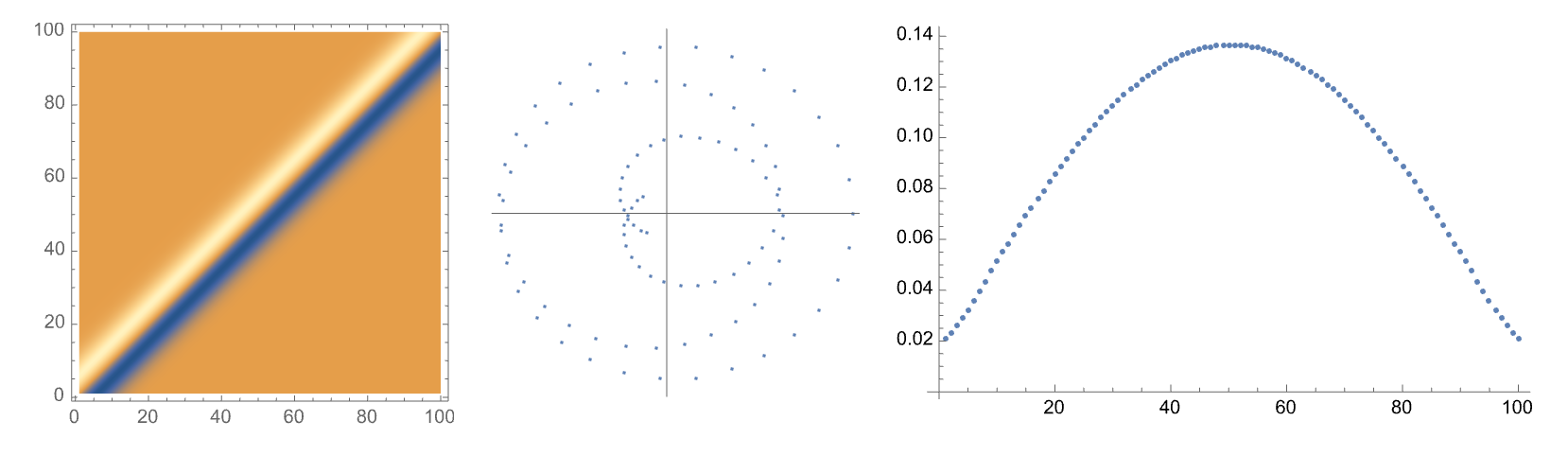
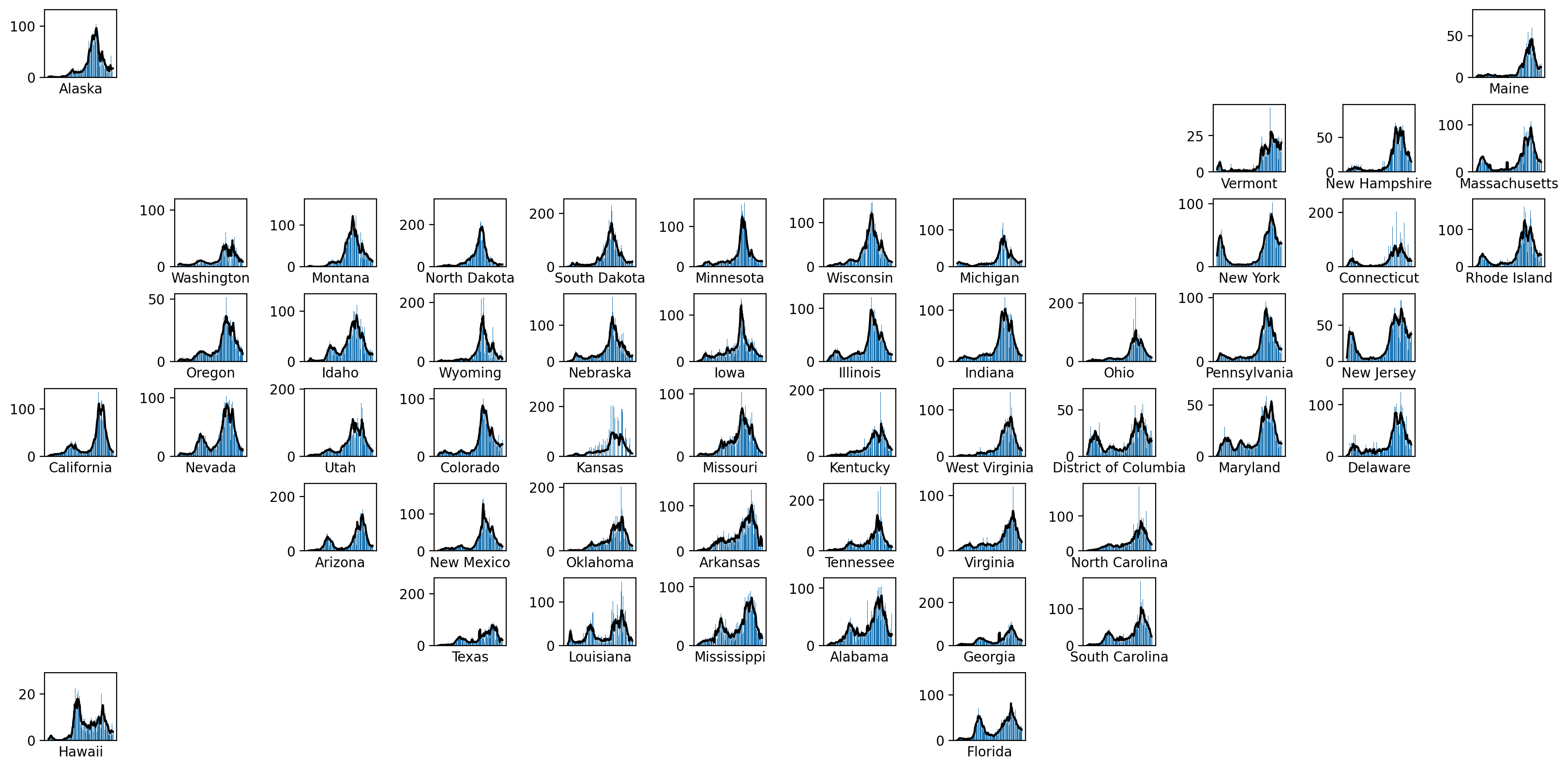
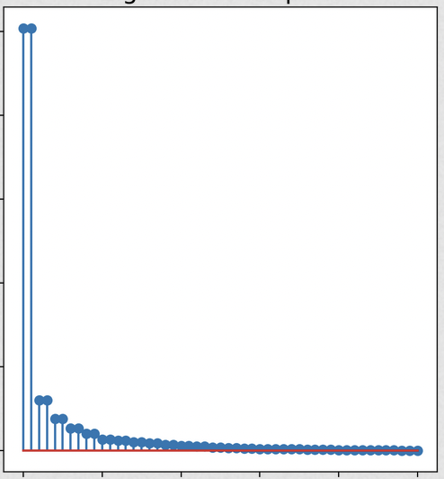
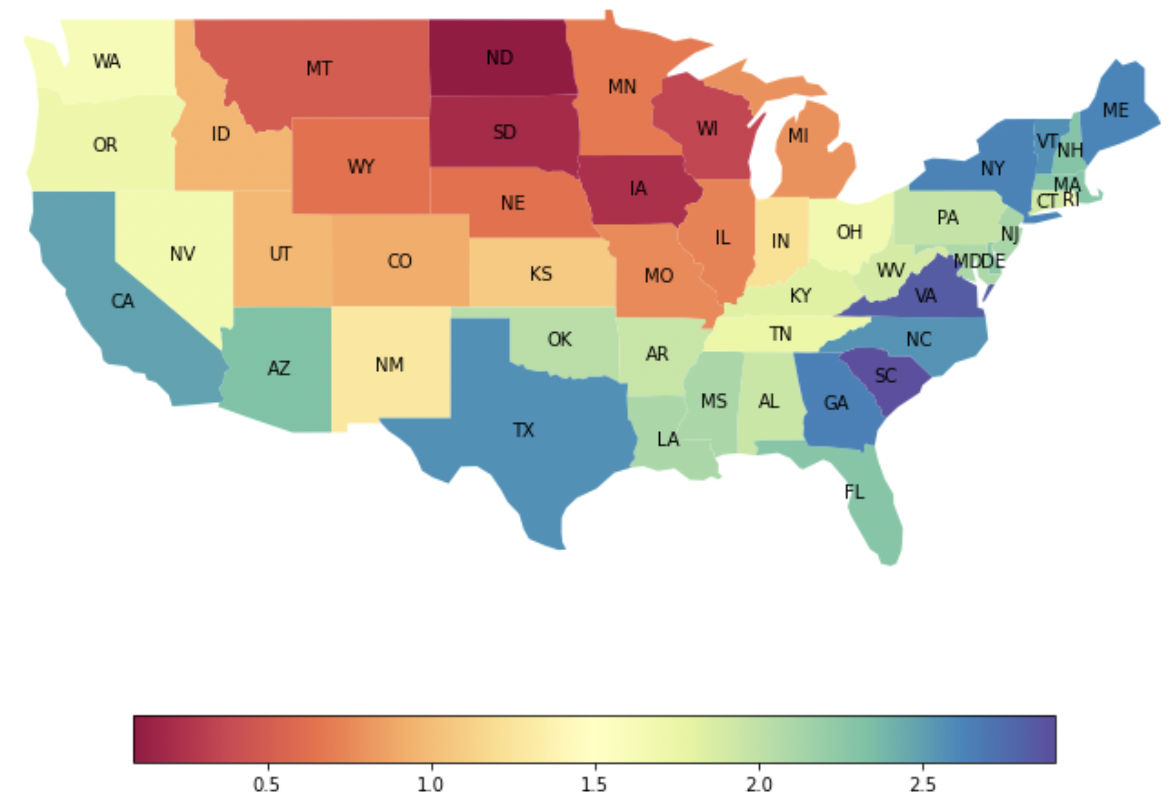
We used the cases per popuation data at the states level. The time interval in this study is June 18, 2020 to February 8, 2022. We used 7 days rolling average of the prevalence as out time series.

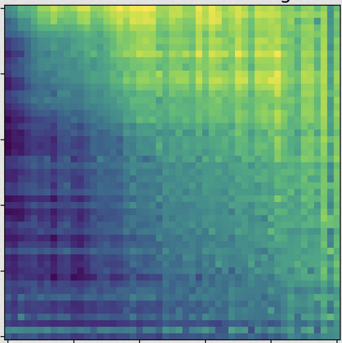
The standard computational pipeline was used.

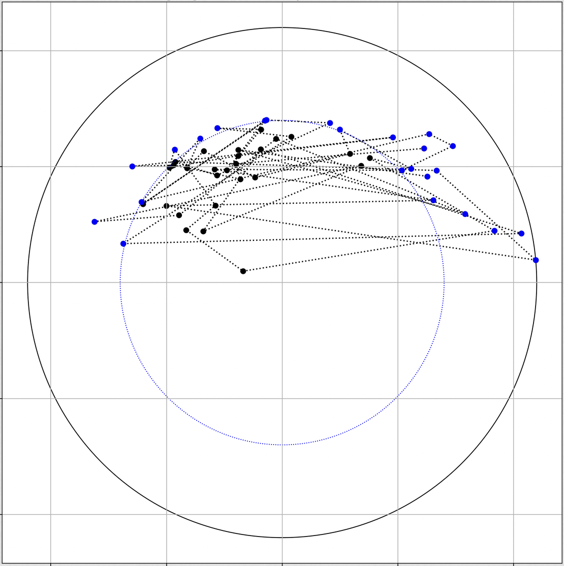
The results are below: the spectrum (showing a dominant mode), sorted lead matrix, convincingly banded, constellation:

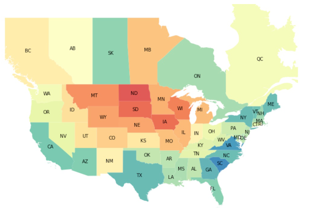
Here the choropleth showing the phases of imputed epidemic propagation (from red to blue):

Adding Canadian provinces indicates discontinuities at the border...

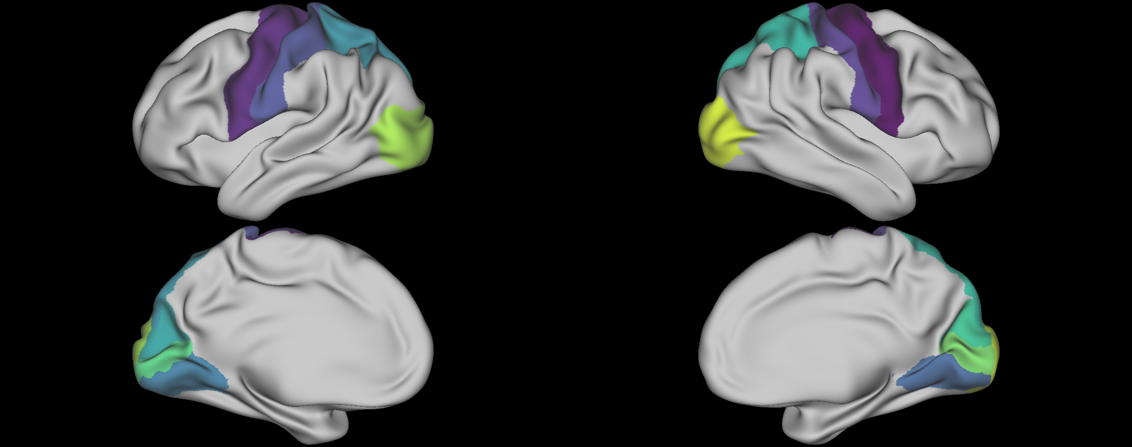
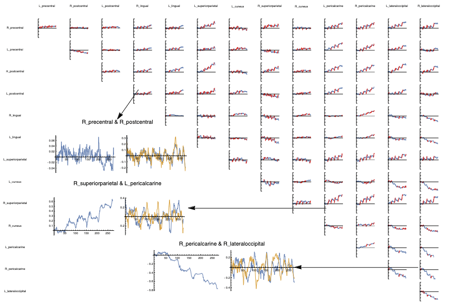
Arrival of functional brain MRI allowed relating activities in different regions of the brain. The notion of Connectome (introduced by O. Sporns)addresses the network structure of such relations, typically derived by correlating simultaneously active ROIs in the brain.

The idea that one needs also to derive temporal relationships between activities of ROIs is being discussed in the community, but the tools are largely ad hoc, relying on approximation and smoothening.

One can think of our lead matrix as the imaginary part of the connectome correlation matrix.

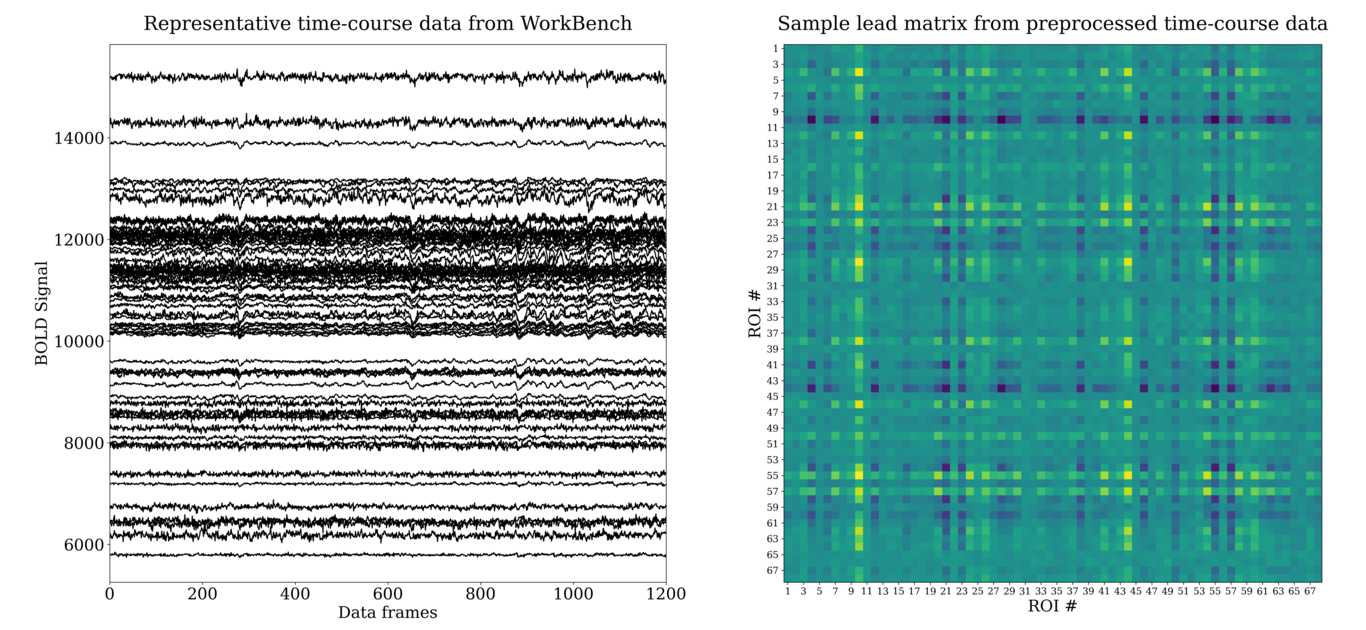
Data: Human Connectome Project 1200 Release $\Rightarrow$ 862 de-noised minimally preprocessed participants with resting state, and task fMRI sessions using a customized Siemens Skyra 3T scanner. We extracted time series from regions of interest (ROI) information in the fMRI parcellations available for download.

We aggregated the voxel level data into 34 pairs of symmetric ROI, scanned at $1/720$ ms, and put the resulting time series through out pipe.

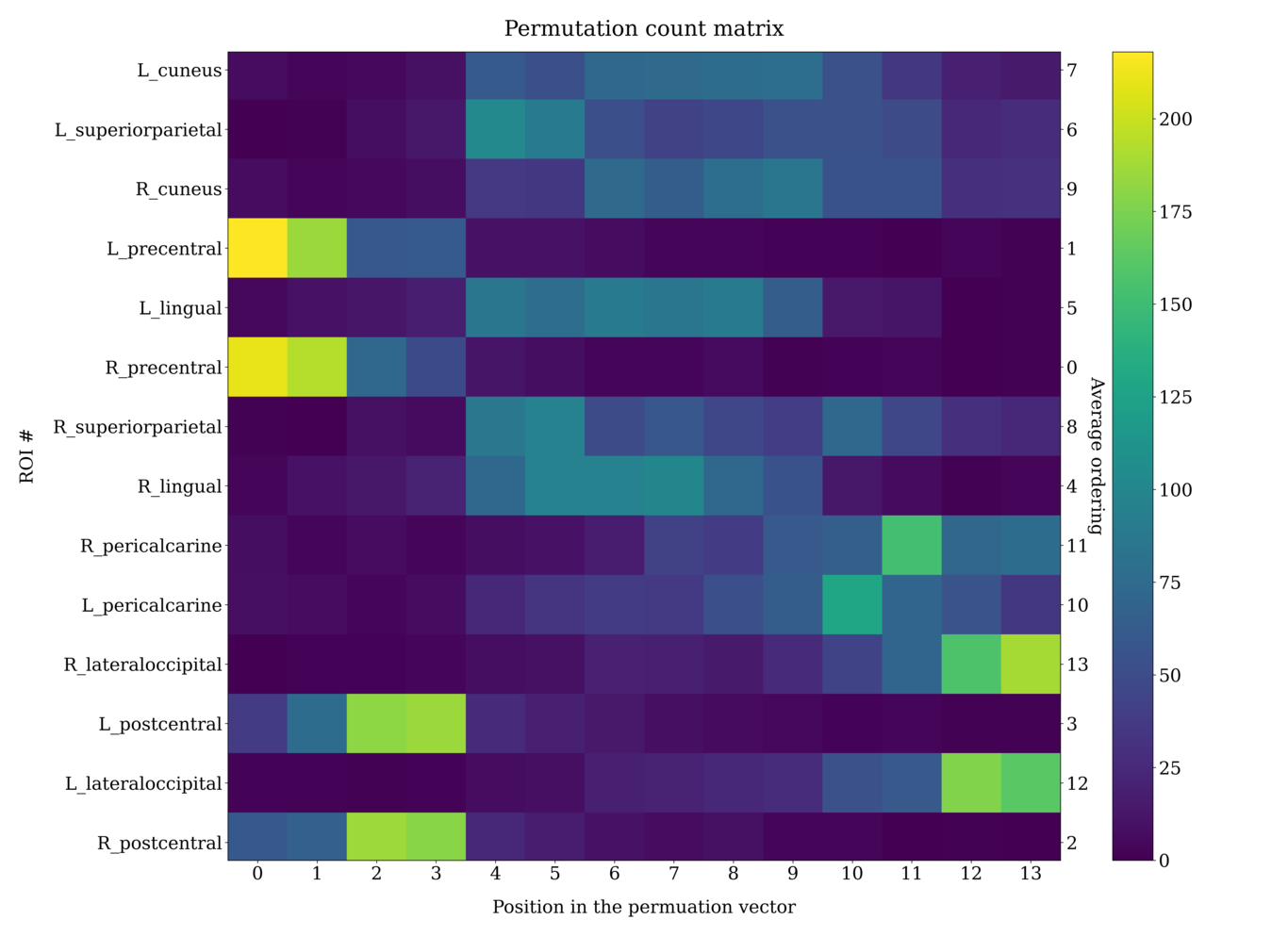
The number of ROIs we started with was high, so we decided to focus on the 14 regions that were consistently strongly represented on constellation plots.

These regions cluster themselves into a clear sequence, indicating the presence of a consistent slow wave traversing the cortex in the resting state, at subHerz frequency.

Remarkably, it seems that in some tasked situations, the direction of this wave reverses.

Success story of a data analysis tool is a function of the tool and the data.

The Cyclicity pipe we created shows some highly nontrivial outputs, which we still learn how to interpret.

This work was done with Emily Schlafli, Ivan Abraham, Vikram Vamavarapu, Dr. Fatima Husain.

THANK YOU!